YouTube has been the leader among content creation platforms for decades, witnessing a surge in the variety of uploaded content. YouTube demands creators to showcase their talent and optimize their content to increase the number of views, ultimately maximizing its reach. This research aims to determine the most crucial factors in boosting the number of views, with a primary focus on elements presented to users - specifically, thumbnails and titles (refer Fig. 1). While video content, watch time, likes, shares, and subscribers play significant roles in YouTube's video recommendation system, this study examines whether titles and thumbnails have a noteworthy impact on converting a video recommendation into an actual view.
The author's previous research establishes that titles indeed play a role in influencing views. The study observed that shorter titles gained more traction compared to longer ones. The current study aims to build upon this research by extending the idea of titles' influence on views and incorporating the characteristics of thumbnails. In the journey also explore the other performance metrics such as likes, subscribers and number of comments on a video and its relation to title and views.
 Fig. 1 Youtube video format
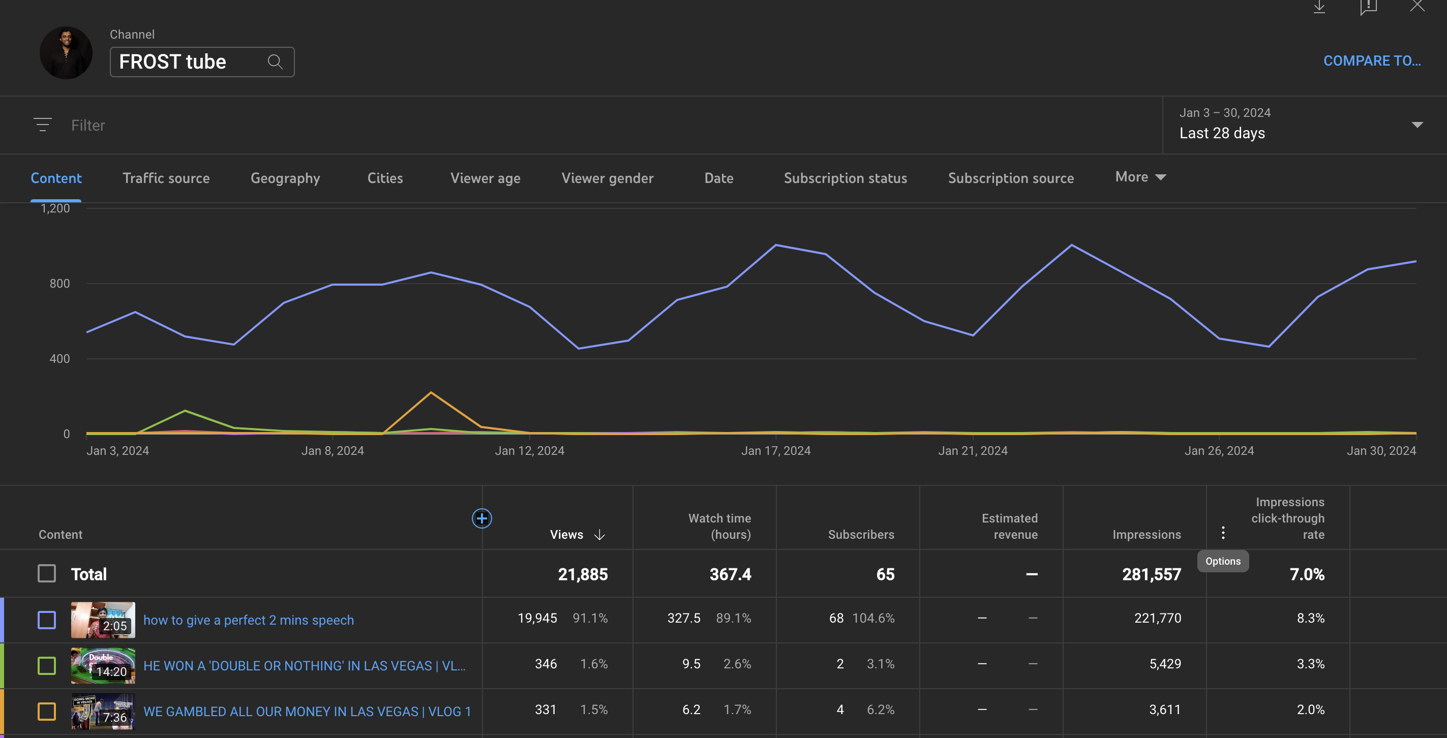 Fig. 2 Youtube Analytics
YouTube Analytics Application is a platform (Fig. 2) created by Google for YouTube content creators to analyze their data. It displays basic analytics such as the number of views, shares, likes, dislikes, subscribers, and click-through rate. Additionally, it provides content creators with the freedom to visualize their data to gain more insights into the relationship between variables. The platform offers in-depth analysis of video performance, aiding content creators in improving video quality and content. Despite these features, there is currently no tool or analytics within the platform specifically designed to help creators craft effective titles and thumbnails – a critical aspect of content creation.
Several studies have examined the impact of YouTube thumbnails and titles on views and video performance. Cheng et al. (2015) demonstrated that both titles and thumbnails significantly influence video views, with thumbnails being slightly more influential. Cheng et al. investigated the impact of YouTube metadata on views using statistical analysis rather than applying machine learning concepts. Koh et al. (2018) emphasized the importance of visually appealing thumbnails in enhancing video performance over time. Their study suggests that creating visually appealing thumbnails does indeed impact video performance, as visually appealing videos were observed to perform better. The study also employed a statistical approach to understanding the impact of thumbnails on views. Dong et al. (2024) conducted research similar to Koh et al. to study the impact of visually appealing thumbnails on views. They observed a significant correlation between thumbnail design and video metrics, notably emphasizing the positive impact of a distant background, focusing on one person, and using concise headings. Similar to the other papers, this study approached the effect through a statistical analysis standpoint.
The focus of this research is to develop a tool that assists content creators in evaluating the quality of their titles and thumbnails. Additionally, the research aims to understand the impact that titles and thumbnails can have on users' mindsets, influencing their decision to either click or ignore the video. The fundamental question regarding the influence of titles and thumbnails on views leads to several intriguing research inquiries, outlined below. The project aims to shed light on the types of sentences and images that attract human attention, thereby affecting the click-through rate. This understanding could prove valuable across various domains, such as advertising, enabling brands to comprehend the impact of the text and images they employ in their advertisements and enhance them based on the findings of this research.
Such a tool could aid YouTube content creators in tailoring titles and thumbnails to any category of videos by analyzing their effectiveness in gaining traction and ultimately popularity on the platform. Though the tool does not guarantee success on YouTube, it assists in ensuring that visible aspects to the audience are tailored according to their needs, potentially increasing views. Research in the field of the impact of titles and thumbnails on views is not only important for creating a tool to enhance content creators' channel views but also for understanding the psychological impact of text and images on human behavior and its influence on video click-through rates. Understanding these psychological aspects could lead to the development of stronger advertising and marketing models.
Through this approach, the model seeks to gain insights into the human mindset, specifically addressing the question: 'What prompts a user to click on a YouTube video once recommended?' Breaking it down into 10 research questions,
The research questions stated above should give a deeper understanding of the underlying reasons behind viewer engagement and the intricate dynamics influencing the success of YouTube videos. The data collected to analyse and answer the above questions are collected from various sources. The following section will examine the data collection process,
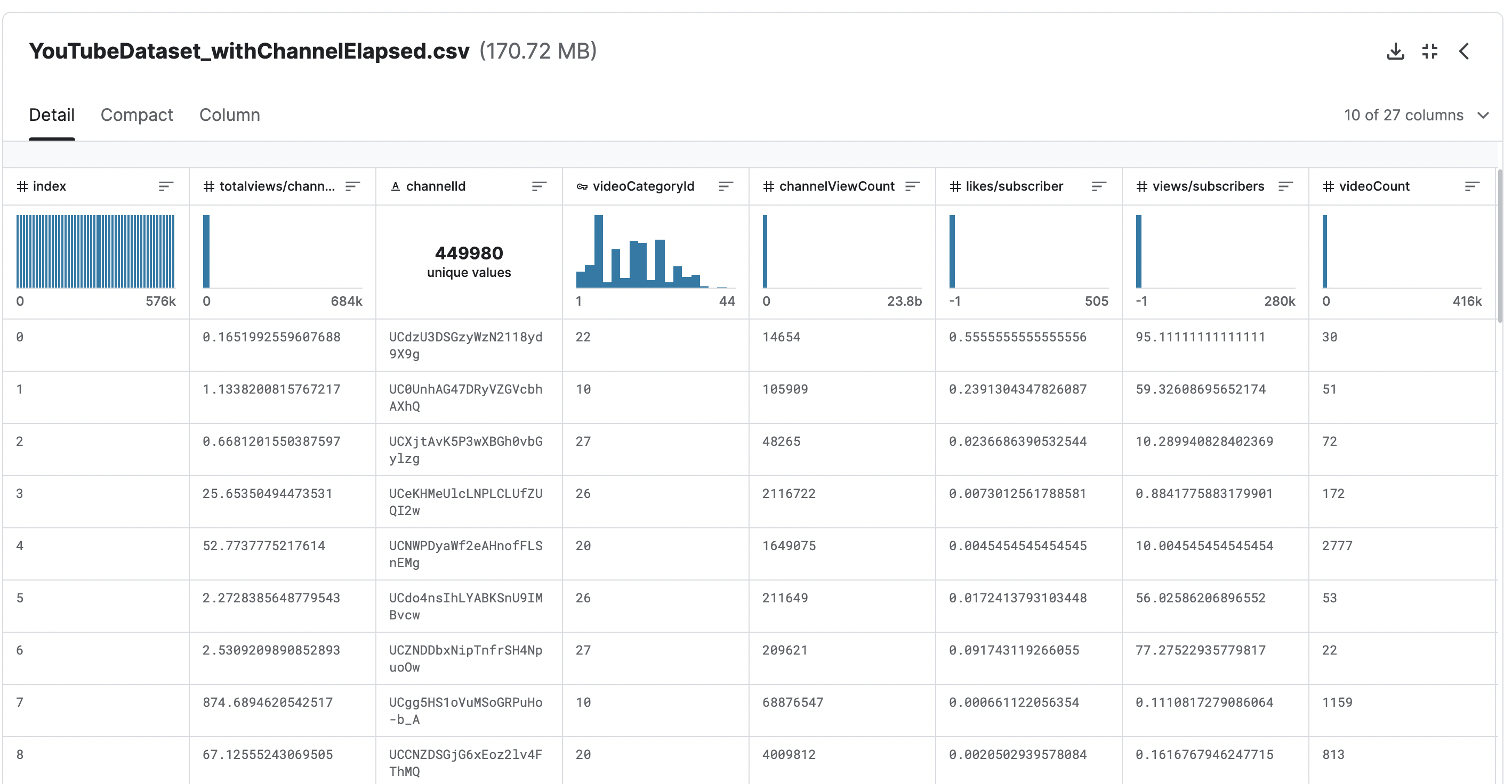
The major chuck of data that has been utilized in this project has been taken from Kaggle, uploaded by VISHWANATH SESHAGIRI [source]. (Click on the image below to view it in a seperate tab)
Youtube API was utilized in collecting youtube title information given the video ID. Title is one of the most essential components of the data. (Click on the image below to view it in a seperate tab)

Youtube API was utilized in collecting video thumbnail URLs given the video ID. Thumbnail is another really essential components of the data [Source code]. (Click on the image below to view it in a seperate tab)
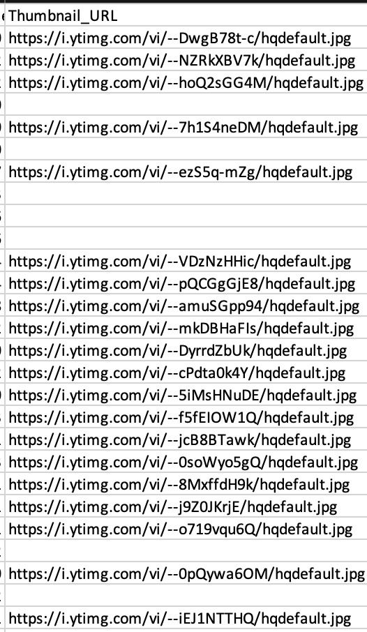
API is used to download the images from the thumbnail URLS, the downloaded thumbnails are stored into a google drive link [Final uncleaned data]. The total time taken to collect 100k titles and thumbnails was 7 days. The API data collection will continue to fetch at least 300k data points. (Click on the image below to view it in a seperate tab)

This section will take you on a journey in understanding the underlying data and cleaning it for analysis and modeling
To initiate a comprehensive understanding of the data, a word cloud (refer to Fig. 3) has been generated to provide an overview of the columns present in the dataset. It should be noted that the word cloud was created to emphasize words with higher repetition. It is evident that several 'Unnamed' columns may have been generated while storing data using an API key; these should be removed. Additionally, the 'index' column serves no purpose and can be excluded. Other columns should be retained for further analysis. Moving on to analyzing the amount of missing values in the most important columns of the data.
 Fig. 3 Column names word cloud
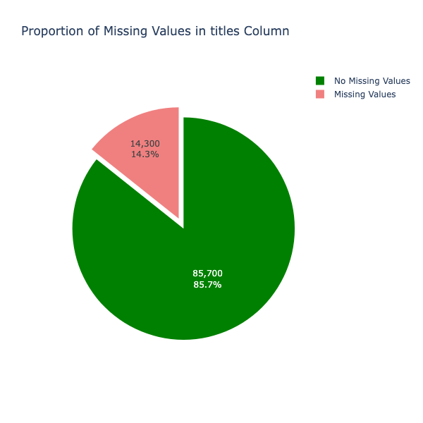
Fig. 4 Proportion of missing values in titles column
After some cleaning, it is observed that none of the columns have missing values. To proceed with data preparation, a deeper examination of the columns is required. The following section will focus on the most important columns and aim to clean them, completing the data cleaning process.
The video view count (Refer Fig. 6) seems to follow a exponential distribution, to understand the distributions better, the histogram for the views under 8k views is plotted. It should be noted that there is a data point that falls below 0, which is not plausible as views cannot go below 0. This issue will be resolved by removing the single row containing this anomaly.
The histogram for views under 8k (refer Fig. 7) reveals that the majority of records fall within the bracket of 0 to 4000 views. To build a classification multimodal, achieving a more balanced distribution of data across various view brackets is essential. This aspect will be addressed in the upcoming sections of the research, where additional data will be collected to ensure a more even distribution.
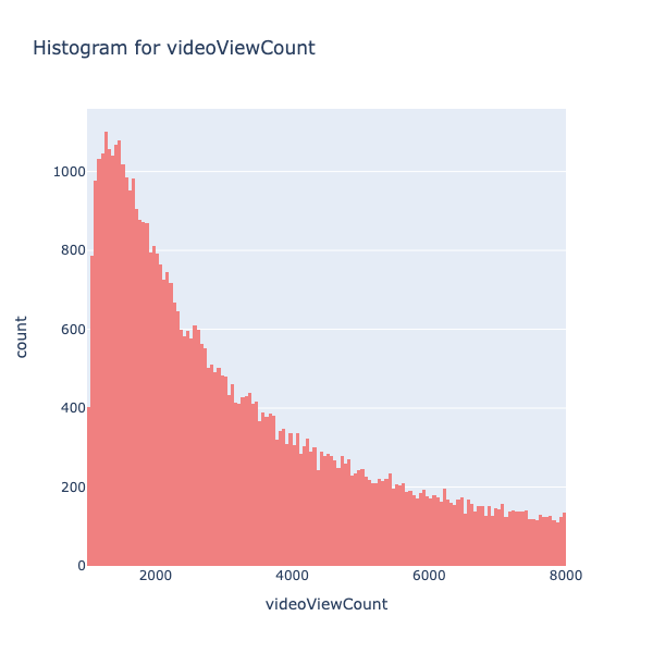
Fig. 7 Histogram for video view count (zoomed in)
The box plot (Refer Fig. 8), although not providing detailed information about quantiles, primarily focuses on identifying outliers. It is observed that the dataset contains numerous outliers, with some particularly significant ones having a view count exceeding 50M. Notably, there are very few videos with more than 50M views. The potential impact of these outliers on the analysis will be assessed after collecting more data to determine if this pattern persists.
One of the more intriguing columns to observe is 'views/elapsedtime.' This column interprets views not merely as raw data but as a variable that changes over time. It aids in understanding whether a video gained views steadily over the long run or experienced immediate effects, and vice versa.
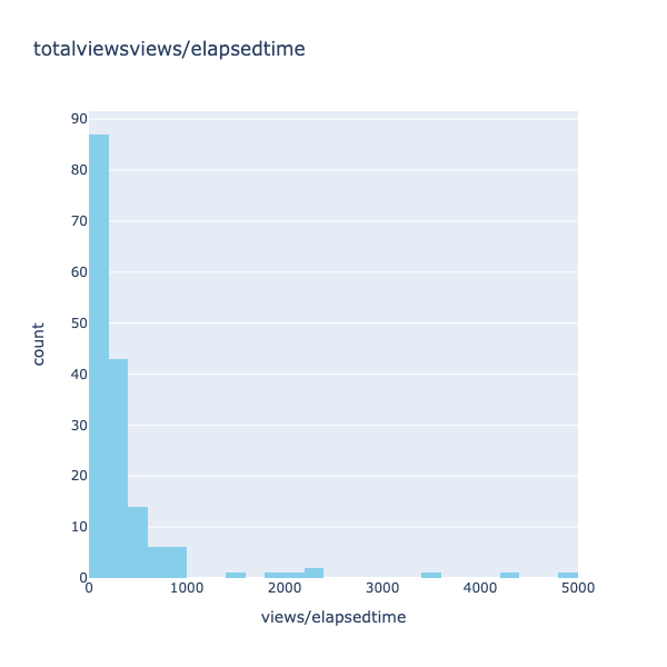
Fig. 10 Distribution of the views/elapsed time (zoomed in)
It is interesting to note that there are numerous videos with views exceeding the time elapsed by a factor of 100 to 5000 (Fig. 10). This is a notable observation, suggesting that these videos gained traction very quickly, possibly due to a higher number of subscribers on the channel. The audience's immediate interest in upcoming videos could explain the rapid viewership. However, as our focus is on assessing the impact of titles and views on overall viewership, such cases may not accurately represent the relationship. Consequently, these rows will be removed from the dataset.
The data interestingly spans across the majority of YouTube categories (Fig. 11 and Fig. 12), exhibiting an almost equal distribution among key genres such as entertainment, people and blogs, gaming, and sports. It should also be noted that most of the genres have more than 2000 vidoes in the data containing 100k data points. This diversity is beneficial, as modeling the data can provide insights into the impact of titles and thumbnails not only within a single category but across a wide spectrum of categories.
At this point, the data is more or less clean, exhibiting no missing values and featuring appropriate data types with consistent values. While the dataset contains some outliers, they are retained at this stage as they might prove useful for the subsequent analysis. A partial snapshot of the cleaned dataset is displayed below (refer Fig. 13x). The image illustrates an additional column that has been introduced (VideoCategory), along with cleaned titles and thumbnail URL columns.
The two plots (Fig. 4 and Fig. 5) depict the number of missing values for the columns 'titles' and 'Thumbnail_URL'. It is observed that after the API data collection for 100k data points, almost 14% of the data had missing values. Removing rows with missing values is essential, as rows lacking the most important features for the research are practically not useful. The number of videos could be increased by collecting more data using the API, a step that will be taken in the further sections of the research work.
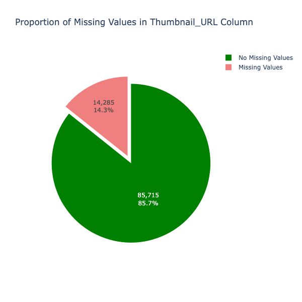
Fig. 5 Proportion of missing values in thumbnail URL column
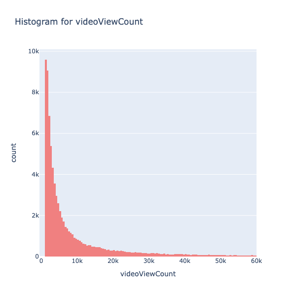
Fig. 6 Histogram for video view count
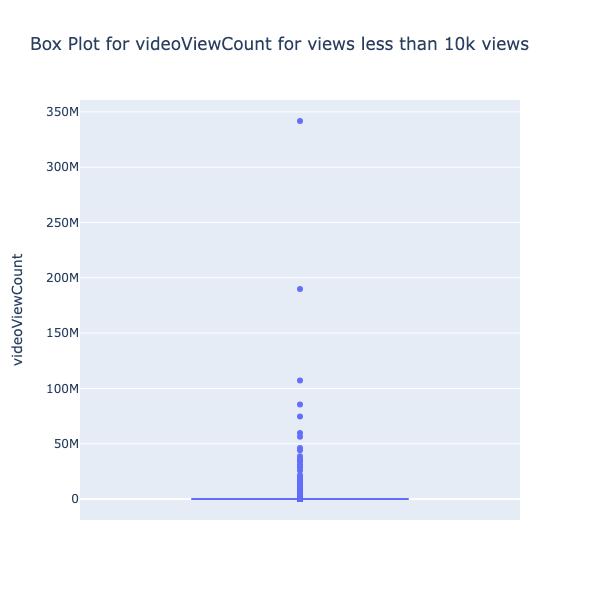
Fig. 8 Box plot of video view count
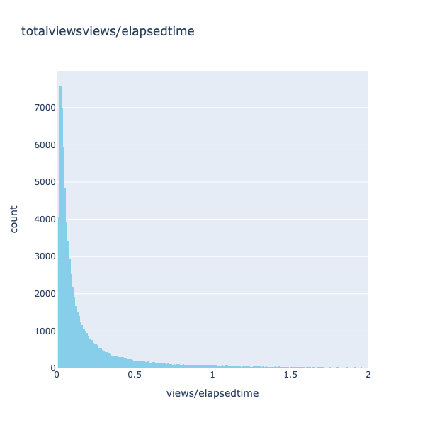
Fig. 9 Distribution of the views/elapsed time
From Fig. 9, it must be noted that most of the values lie in the range of 0 to 1, which means that most of the videos present in the data has views less than the time elapsed after posting the video. Which is obvious as majority of the videos lied in the view brackets of 0 to 4k and mostly channel elapsed time woud be greater than the number of views the video gained. But the intesting points are the ones from 100.
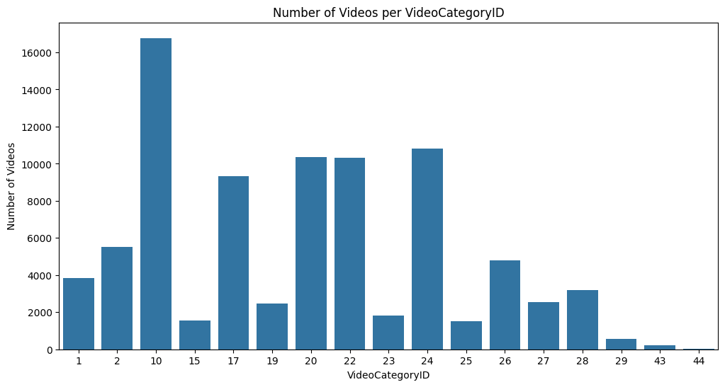
Fig. 11 Videos per video categoryID
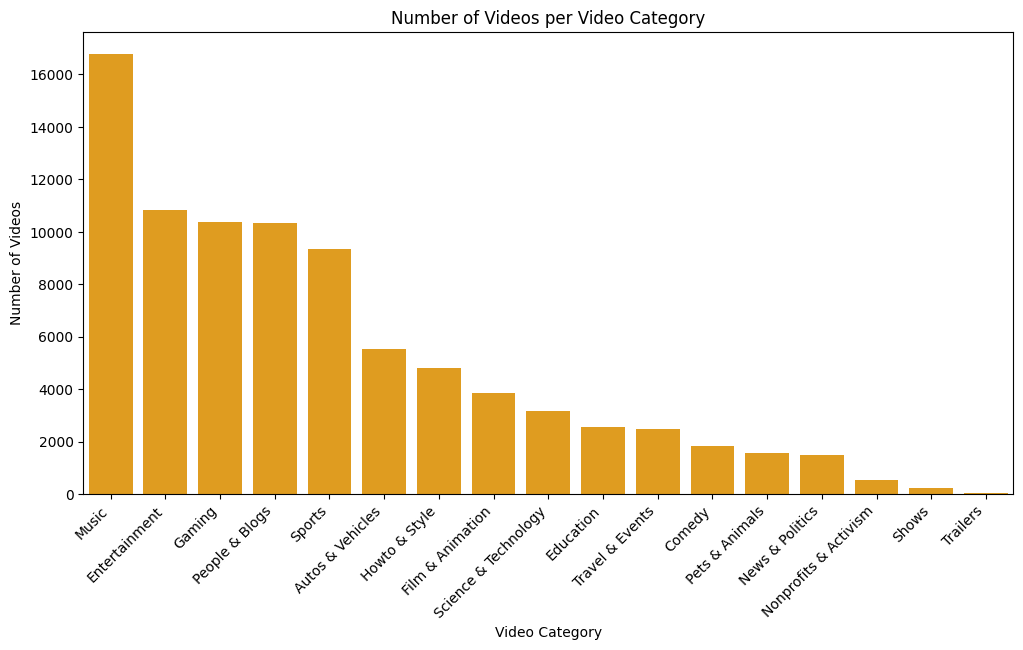
Fig. 12 Videos per video category
From prior research, the relationship between title length and views suggests that title length does play a role in influencing the number of views a video gains. Though the relation is not directly causal, it could be said that title length does influence views. To confirm this hypothesis, k-means clustering is performed on the data. K-means clustering is a form of unsupervised learning which helps in deriving the clusters of data that are related to one another by using a distance metric. The distance metric used for this method is the Euclidean distance. Euclidean distance takes into consideration the shortest distance between data points and thus helps in finding the closest points. The formula is provided in Fig. 14. K-means clustering is a form of partition clustering which is an algorithm that divides the dataset into sub categories based on certain criteria such as the shortest distance between the clusters and the centroid.
To advance the analysis, titles undergo embedding using a VGG16 network (see Fig. 15) to extract key features from the text. The VGG16 network, commonly utilized for image recognition, is repurposed for text analysis. The title embeddings are then subjected to hierarchical clustering to identify the closest titles. Notably, the 'views' variable is not utilized in this method. Hierarchical clustering offers advantages over k-means clustering, as it does not require a fixed number of clusters to be specified, allowing for the natural structure of the data to emerge. The approach employs divisive clustering, where each data point initially forms a single cluster and subsequently divides into smaller clusters. The distance metric utilized for this method is cosine similarity, chosen for its effectiveness in measuring the similarity between embedding vectors (see formula in Fig 16).
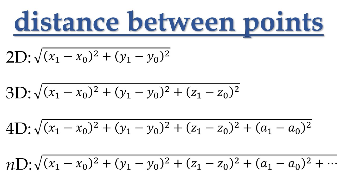 Fig. 14 Euclidean Distance Formula
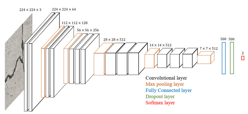 Fig. 15 VGG16 Architecture
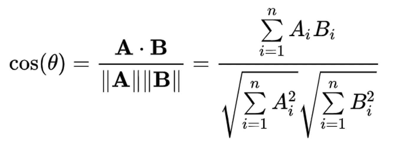 Fig. 16 Cosine Similarity formula
To determine the influence of title length on views, the 'title_length' feature is derived by counting the number of characters in the title, while the 'views/elapsed time' ratio is considered instead of views to focus on the impact of titles relative to the time since publication. The 'views/elapsedtime' column is analyzed for outliers and subsequently removed to ensure accurate clustering. Thus, for k-means clustering, a subset of the dataset containing the 'title_length' and 'views/elapsedtime' features is used (refer Fig.17). Title embeddings are obtained by first passing the titles through a pre-trained VGG16 network with its fully connected layer removed to extract key features. The resulting features are then stored in the 'title_embedding' column. These title embeddings, along with the 'views/elapsedtime' features, are used for hierarchical clustering. Although 'views/elapsedtime' is not directly used in the clustering algorithm, it is utilized post-clustering as labels to analyze the pattern that emerges from the data. The link to the sample data can be found here.
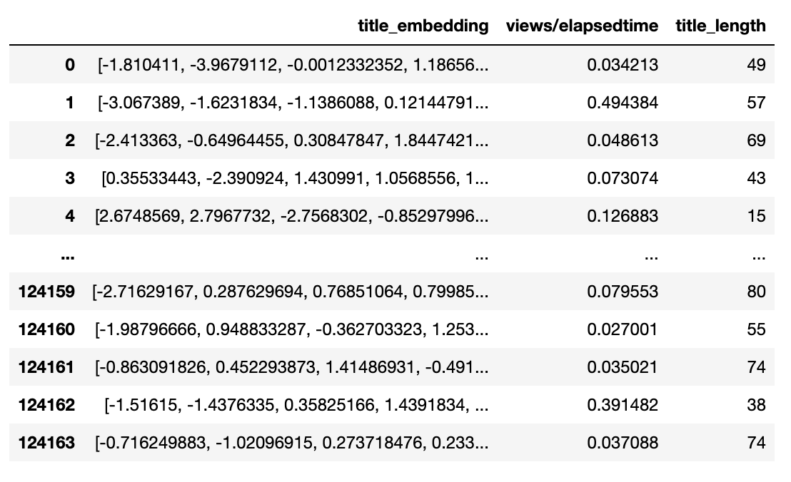 Fig. 17 Clustering Data
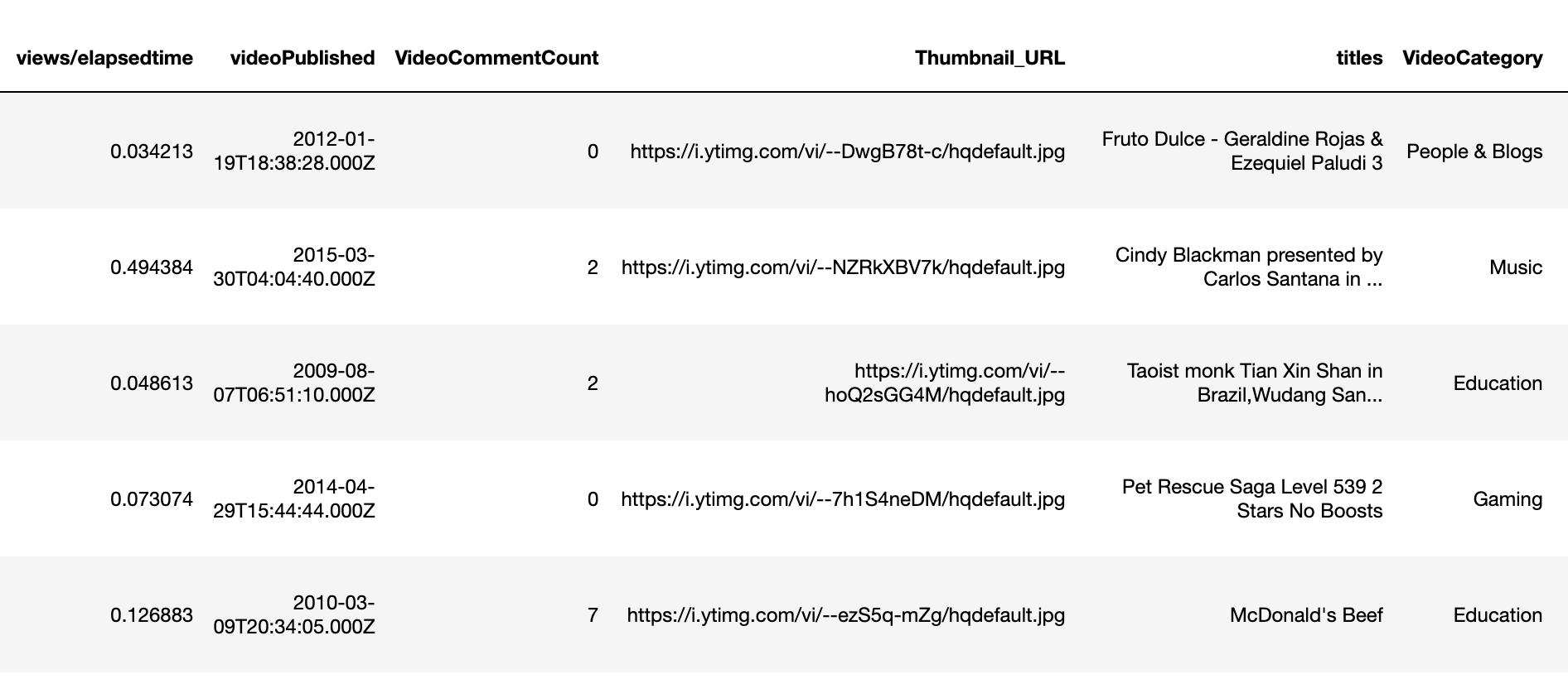 Fig. 18 Sample of original data
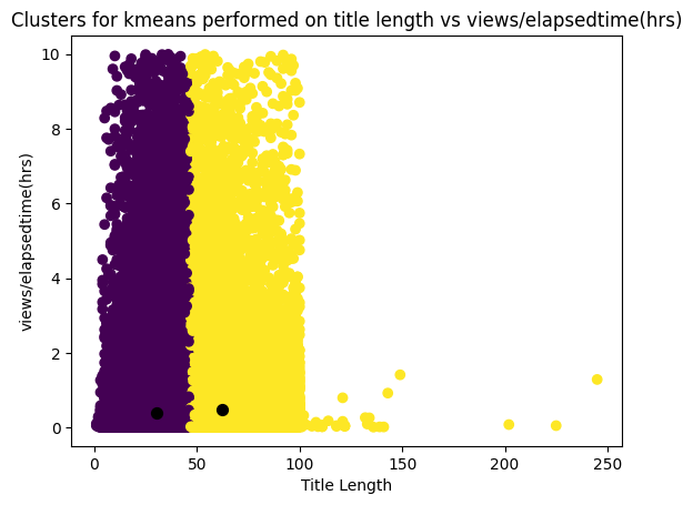 Fig. 21 K-means clustering perfomed for 2 clusters
Three clusters were obtained while clustering the title embeddings. The first cluster primarily included titles resulting in low 'views/elapsedtime' ratios. The second cluster comprised titles with predominantly high 'views/elapsedtime' ratios. The third cluster yielded mixed results, with a combination of low and high 'views/elapsedtime' ratios.
Comparing Hierarchical and K-means clustering, it can be observed that there exist two clusters (though hierarchical provided three clusters the third one can be ignored as it does not capture the video performance based on views) and the video titles fall into each of these clusters based on its characteristics.
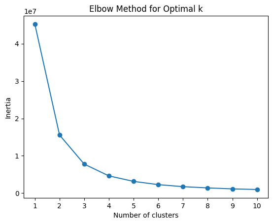 Fig. 19 Elbow method to find optimal K value
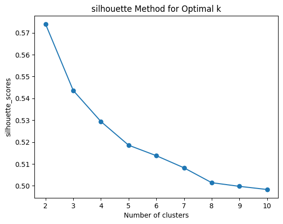 Fig. 20 Silhoutte method to find optimal K-value
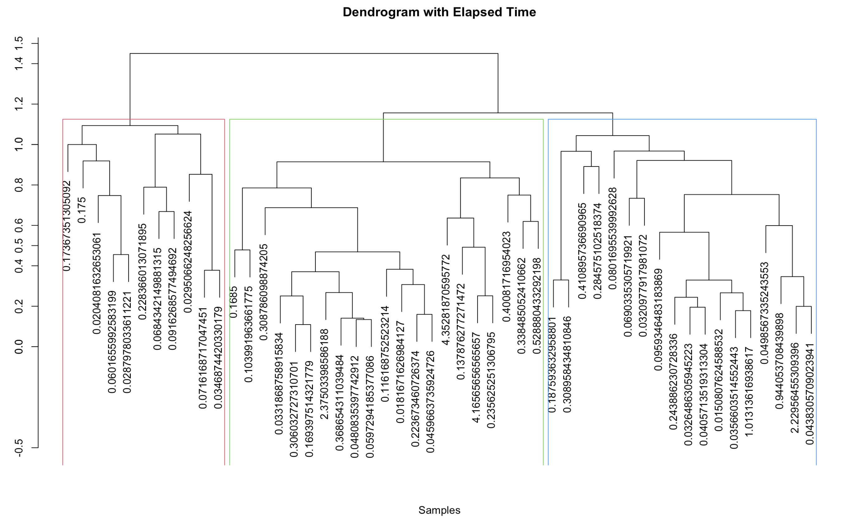 Fig. 22 Dendogram with hclust performed on title embeddings
Based on the results, it is observed that titles with more than 50 characters had a mean 'views/elapsedtime' of 0.5 and a mean title length of 62 characters. In contrast, titles with fewer than 50 characters displayed a mean 'views/elapsedtime' of 0.4 and a mean title length of 30 characters. This suggests that videos with shorter titles performed relatively poorly compared to videos with longer titles. It is worth noting that the boundary lies at 50 characters, and given that the maximum length of a YouTube title is 100 characters, the clusters clearly differentiate shorter titles from longer titles.
The hierarchical clustering revealed three clusters based on title embeddings, each exhibiting varying views-to-elapsed-time ratios. The first cluster displayed a lower mean views-to-elapsed-time ratio, while the second cluster exhibited a higher mean ratio. The third cluster presented a mixture of views-to-elapsed-time ratios. This suggests that titles within the second cluster corresponded to videos with better performance compared to those in the other two clusters.
In conclusion, the results of the cluster experiment indicate that titles indeed have an impact on YouTube video performance.
The conclusions drawn from clustering experiments on video titles and their impact on views suggest that titles indeed play a significant role in video performance. To deepen the analysis, association rule mining (ARM) is employed to study the relationship between title characteristics and various metrics of YouTube video performance. ARM is a method of discovering rules within data to unveil underlying relationships. These rules typically follow an 'if-then' structure, with variables on the left-hand side (LHS) as antecedents and those on the right-hand side (RHS) as consequent (refer Fig. 23)
In ARM analysis, key metrics such as support, confidence, and lift are extremely important. Support indicates the proportion of the dataset containing both the LHS and RHS of a rule, while confidence represents the conditional probability of the consequent given the antecedent. Lift measures the degree of association between the antecedent and consequent, with values greater than 1 indicating a stronger relationship than would be expected by chance.
The Apriori algorithm is used for association rule learning. It is specifically designed to discover frequent item sets in transactional databases and to generate association rules based on these frequent item sets.
This study employs apriori algorithm to investigate the relationship between title length and various metrics of video performance, including views, subscribers gained, comments received, and likes garnered. By analyzing these associations, the research aims to uncover insights into how title characteristics influence video performance outcomes.
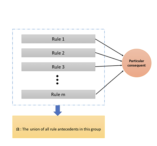 Relationship between antecedent and consequent (Fig. 23)
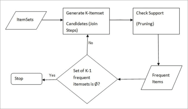 Apriori Algorithm (Fig. 24)
To prepare the data for analysis using the Apriori algorithm, it first needs to be converted into transaction data. The original data, which is in the form of Record data (refer Fig. 25), undergoes a transformation process to create transactional records suitable for association rule mining.
The transformation begins by binning the columns into categories based on an analysis of the data distribution. Each column is processed individually, with the goal of maximizing variability while maintaining equal distribution within each category. For instance, the 'title length' column is divided into 'short title' and 'long title', while the 'views/elapsed time' ratio is categorized as 'performed poorly', 'performed well', and 'performed great'.Other columns are binned as 'relatively more' or 'relatively less' compared to the median of the data. This binning process ensures that each transaction captures relevant information while reducing complexity (refer Fig. 26 for final sample dataset)
In total, approximately 125,000 transactions are generated from the original data. A sample of the final transaction data is provided here.

Fig.25 Sample of Original Cleaned Data
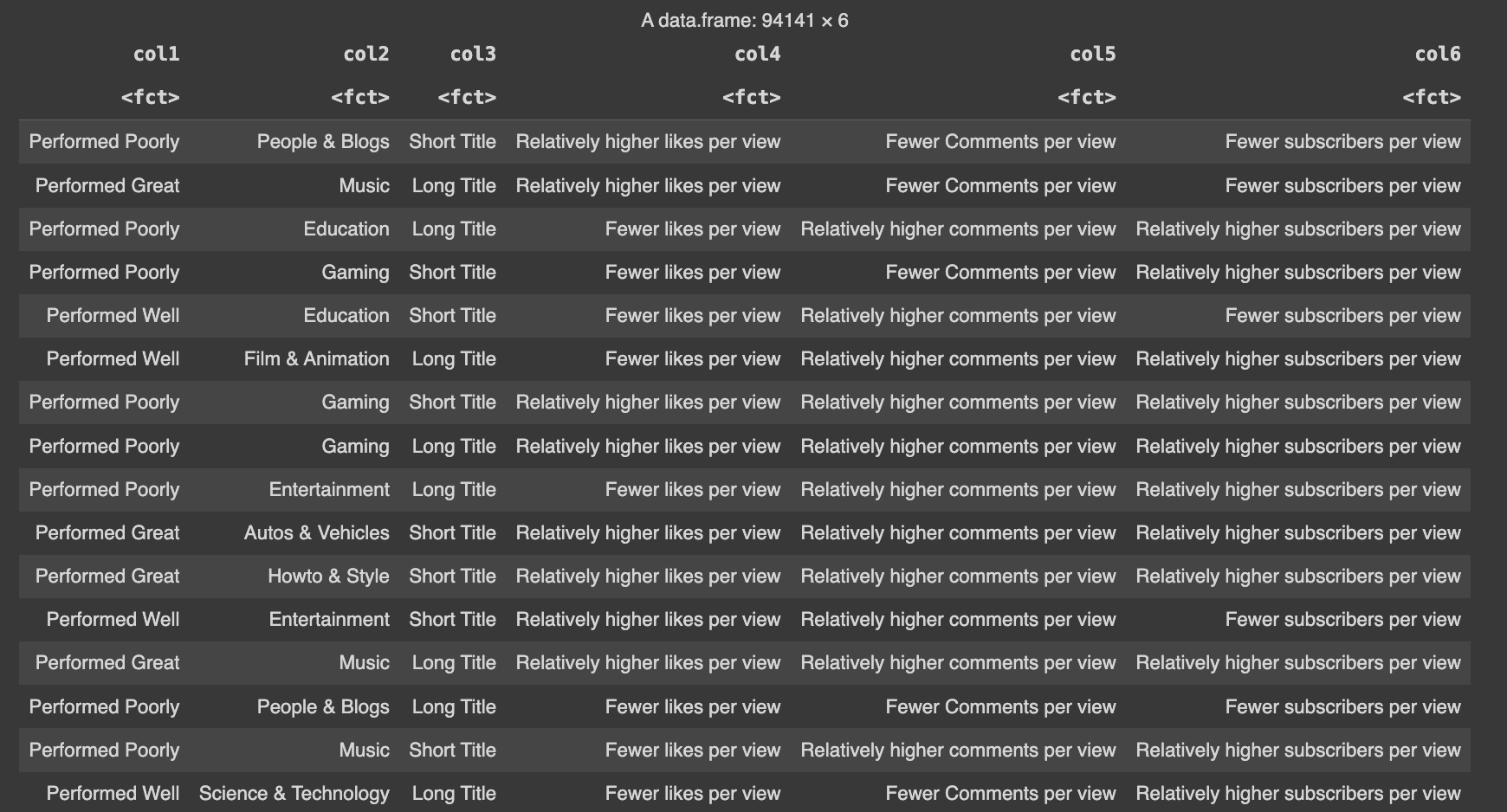
Fig.26 ARM data
The apriori algorithm was run on the dataset to obtain top 15 rules with a fixed RHS of ‘shorter titles’ for support, confidence and lift with a minimum support of 10% and a minimum confidence of 50%. ‘Short titles’ were picked to be fixed as the RHS as it helps in exploring all the patterns that exist around short titles and its impact on the performance of the videos. The rules obtained are as follows:
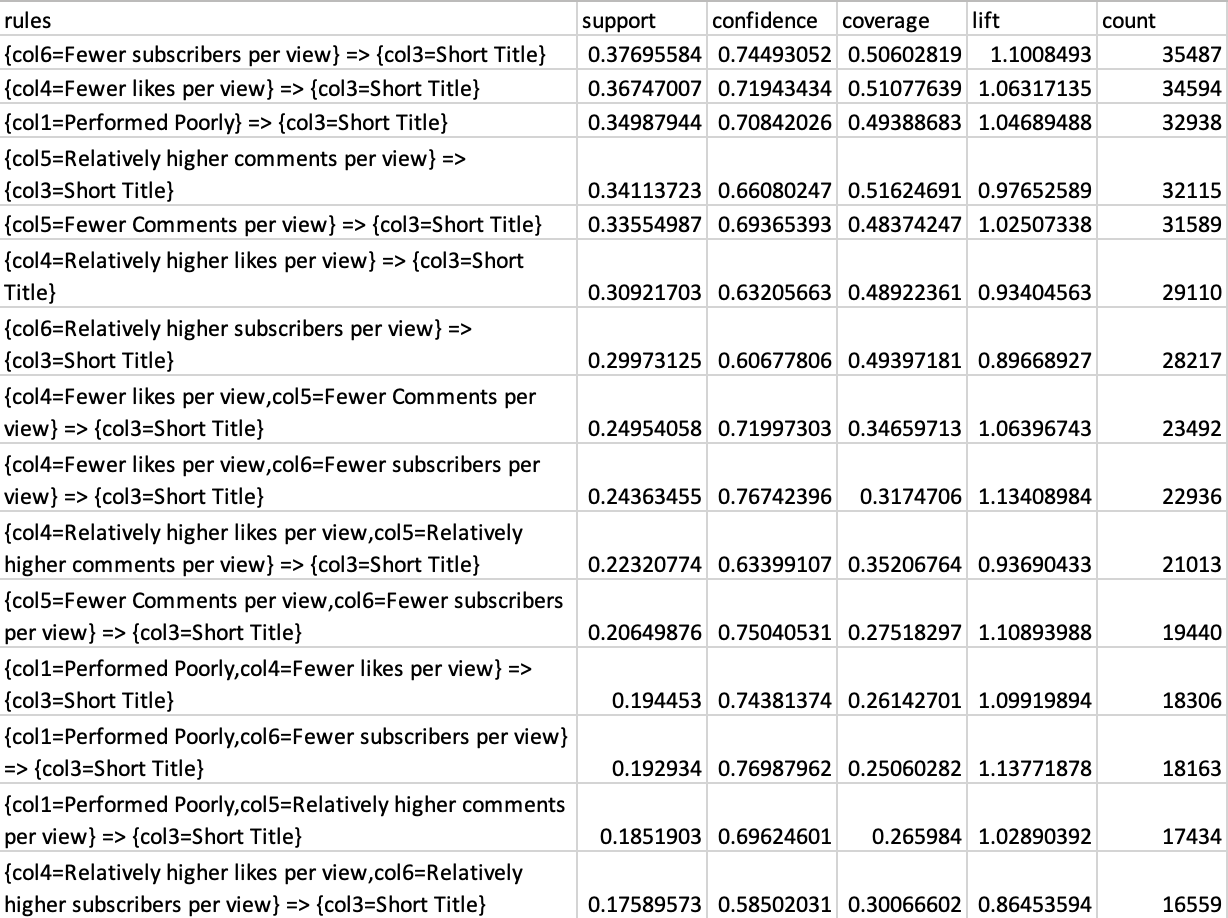
Fig.27 Support Data
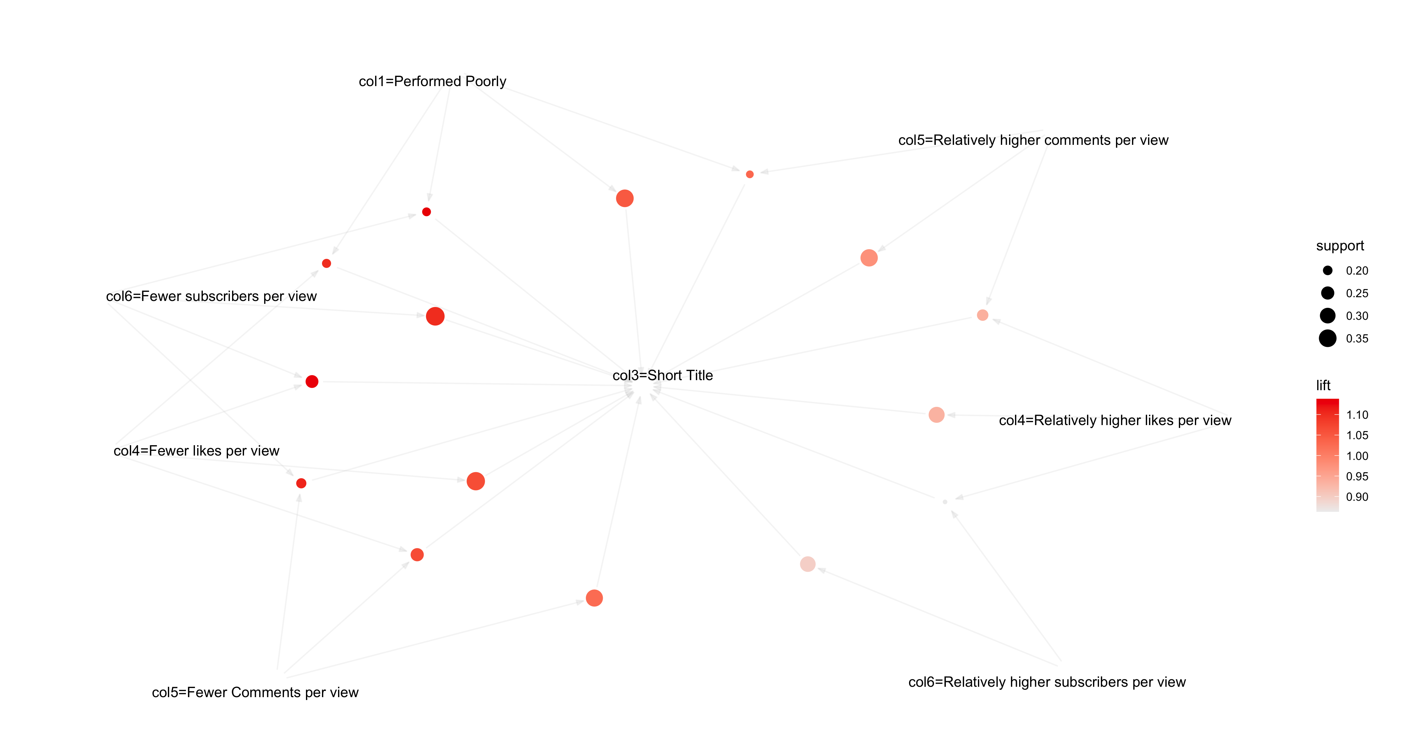
Fig.28 Support rules Visualization
The top rules based on the support metric indicate that videos with shorter titles tend to perform poorly in terms of the number of subscribers, likes, and views they accumulate over time. This observation, with a support of 35%, is significant within the dataset, suggesting a substantial association between shorter titles and lower performance metrics.
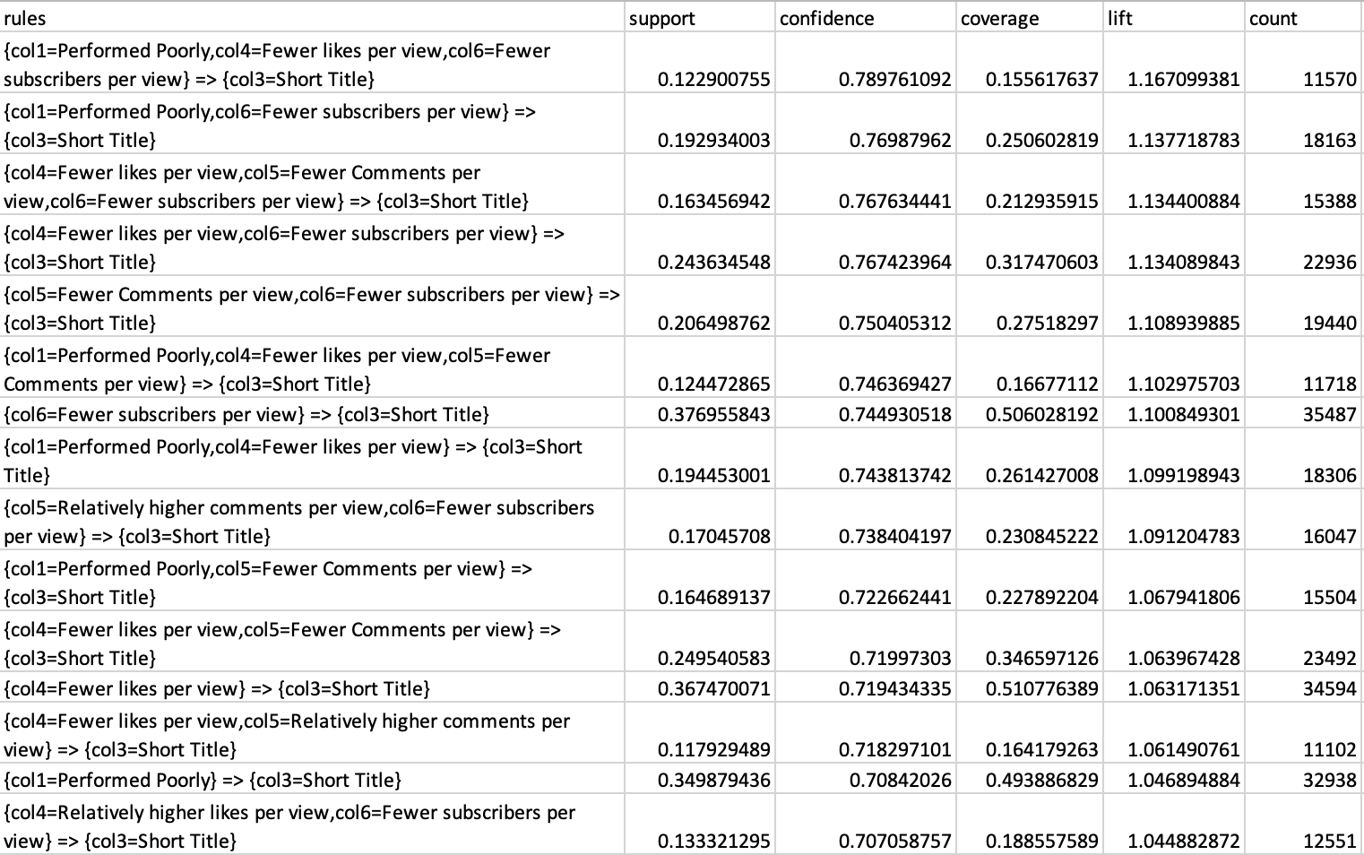
Fig.29 Confidence Data
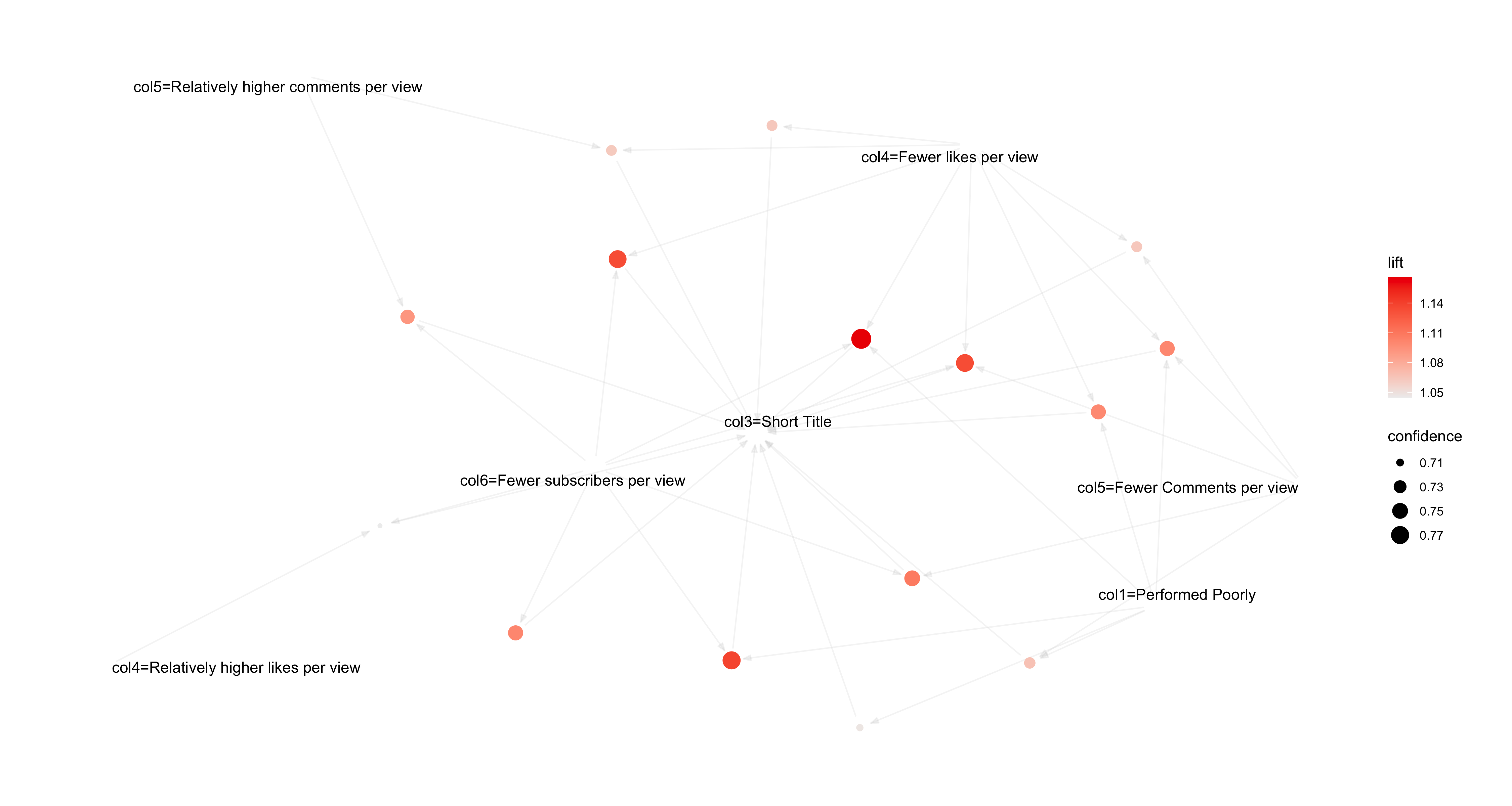
Fig.30 Confidence rules Visualization
The top 15 rules obtained from confidence suggest that similar findings of support, the confidence of the rules signifies that with an average confidence of 75% it could be said that if the video performs poorly, on an average, 75% of the times it consists of a shorter title.
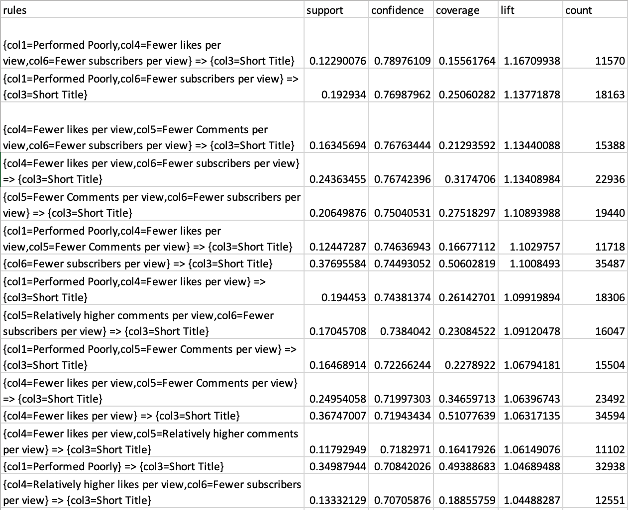
Fig.31 Lift Data
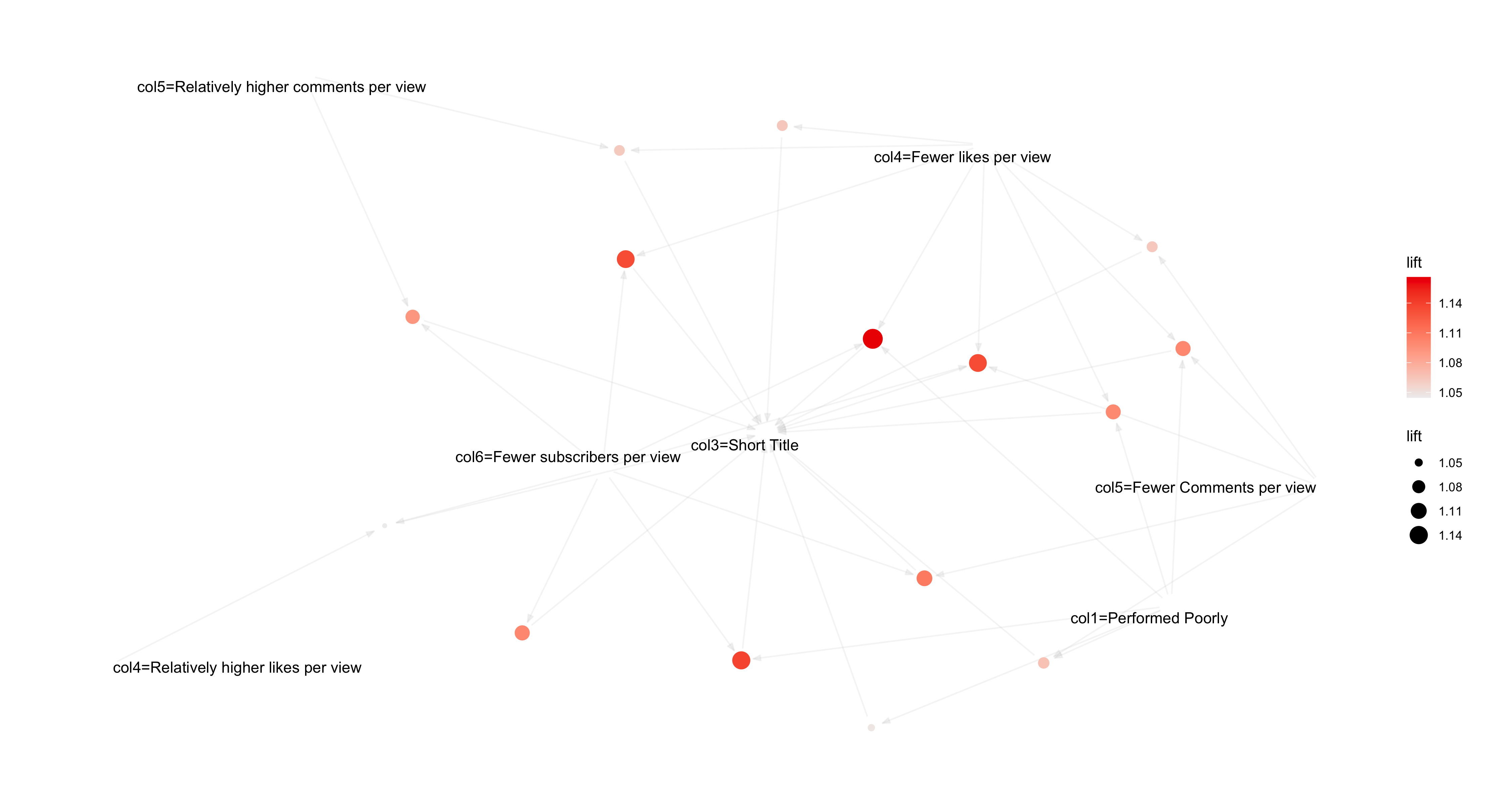
Fig.32 Lift rules Visualization
The higher lift value for the rules also suggests a very strong relationship between the antecedent and the consequent, beyond what could be expected by chance.
From the rules derived through the Apriori algorithm, a strong association emerges between poor video performance and short titles . Notably, an average support score of 30%, confidence level of 70%, and lift value exceeding 1 were observed for rules where poor performance metrics served as the antecedent and shorter titles as the consequent.
The high support, confidence, and lift values confirm that titles indeed impact video views. While the precise magnitude of this impact remains unquantified, the evident relationship between titles and video performance, as revealed by both association rule mining and clustering analyses, cannot be overlooked.
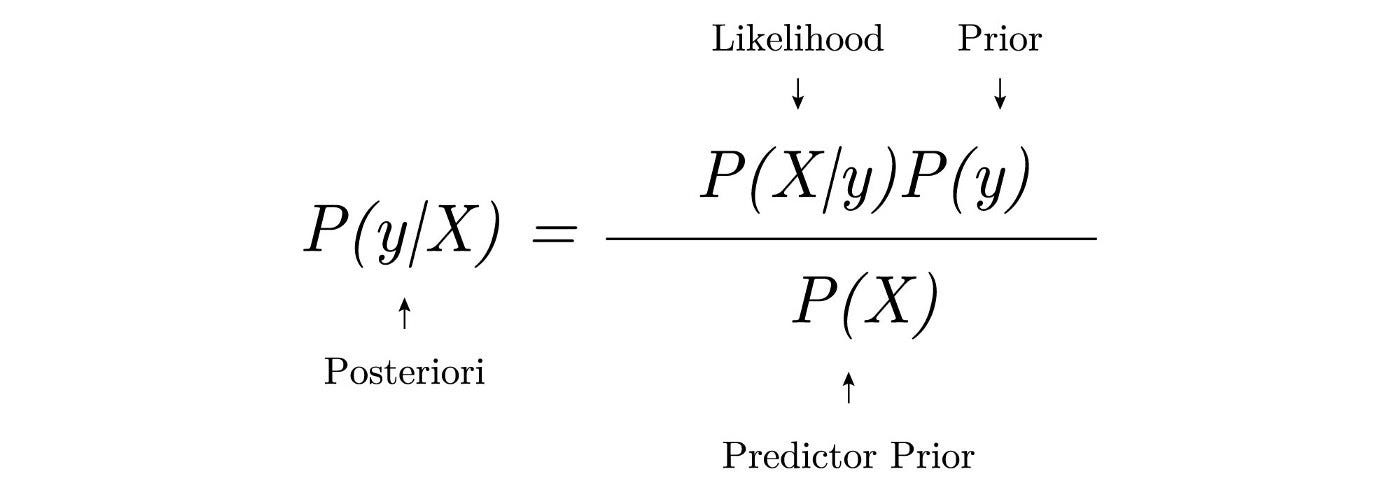
The main principle behind the Multinomial Naive Bayes algorithm is based on Bayes’ theorem (refer Fig. 33), which assists Multinomial Naive Bayes classifiers in determining the probability of a given set of features belonging to a set of classes. Multinomial Naive Bayes is used in scenarios where the data are presented in a categorical format. During training, the model learns the probability of each feature occurring in a given class. This allows it to develop a probabilistic understanding of the dataset. The probabilities calculated during training are then used during testing. This enables the model to predict the likelihood of a given set of unseen feature values and select the class with the highest probability. The Naive Bayes algorithm as a whole assumes independence between features, which is why it earned the name 'naive' Bayes. In this particular project, the Naive Bayes model is used to predict the performance categories such as 'Performed Poorly' or 'Performed Well' based on the given YouTube titles.
Bernoulli Naive Bayes is another variant of the Naive Bayes algorithm specifically designed to handle binary data. It measures the presence or absence of a particular attribute in a dataset. Bernoulli Naive Bayes also makes the assumption that features are independent of one another. This means that the presence or absence of one feature does not affect the presence or absence of another feature. During training, Bernoulli Naive Bayes calculates the probability of each feature occurring or not occurring in each class. It does this by counting the number of occurrences of each feature in each class and dividing by the total number of documents in that class (refer Fig. 34).
 Multinomial Naive Bayes formula (Fig. 33)
 Bernoulli Naive Bayes formula (Fig. 34 )
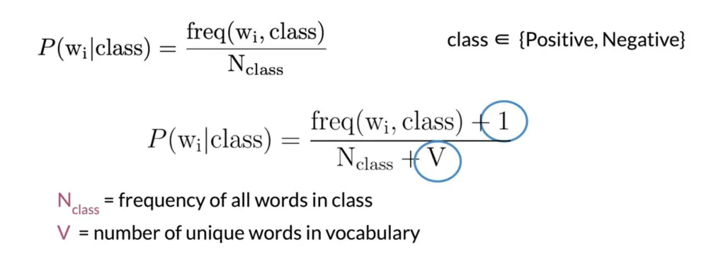 Laplacian Smoothing Formula (Fig. 35)
Smoothing is a process aimed at preventing occurrences of zero probabilities when testing datasets. During testing, there may be instances where a particular feature has no occurrence in the training dataset, while other features may occur simultaneously. This situation would erroneously result in a zero probability for the entire test dataset, despite the chances of occurrence not being truly zero. To address this issue, various smoothing techniques such as Laplace smoothing (add-one smoothing), Lidstone smoothing, or Dirichlet smoothing are employed. By utilizing smoothing methods like Laplace smoothing, we ensure that neither the numerator nor the denominator in probability calculations becomes zero. Fig. 35 provides the formula for the most commonly used Laplace smoothing method.
The data preparation stage of Naive Bayes was conducted in three steps,
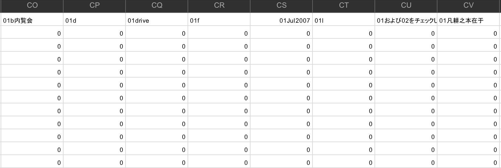
Fig.39 Test data sample
The code to Naive Bayes’ Classifier performed on python can be found here.
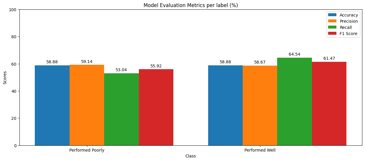
Fig.40 Model Evaluation Metric
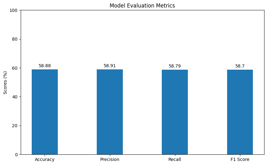
Fig.41 Model Evaluation Metric

Fig.36 Sample of Original Data
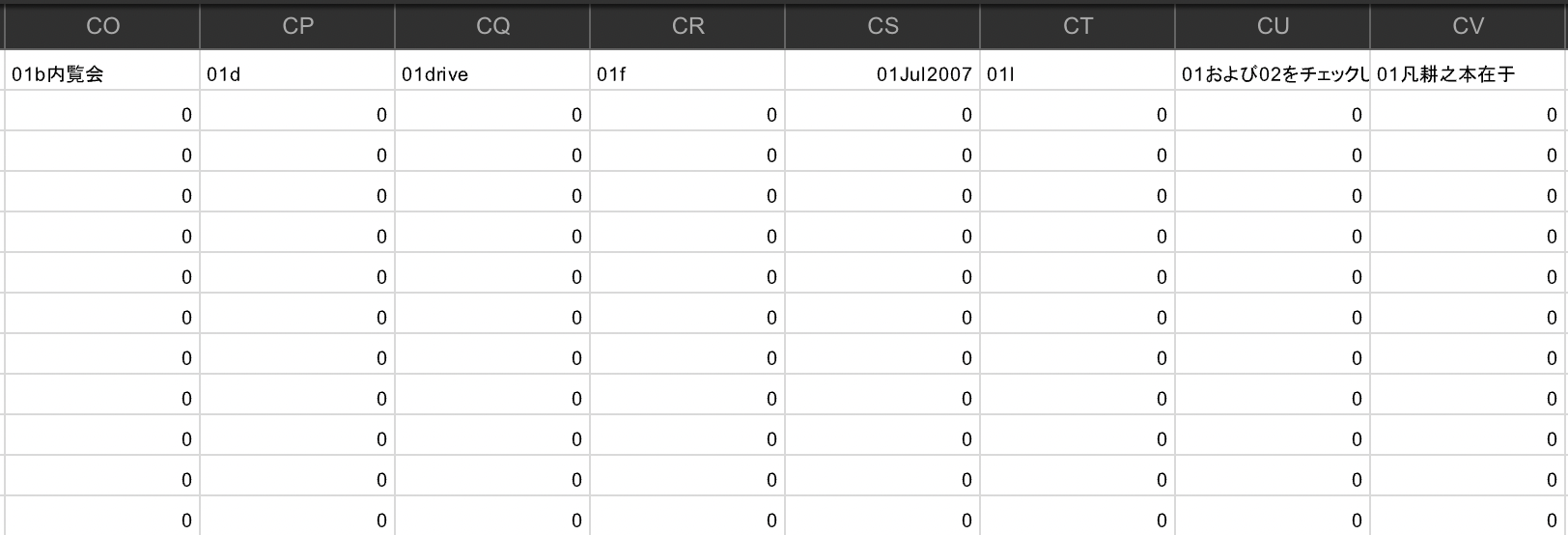
Fig.37 Training data sample
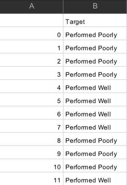
Fig.38 Training data sample
The Multinomial Naive Bayes model was trained on the training dataset with the alpha parameter set to 0.2 for implementing Laplace smoothing. The results were obtained by running the model on the test dataset, as shown in Figure 40. It is evident from the results that both the accuracy and precision of the model were approximately 58% for both labels. However, the recall varied slightly, with the 'Performed Poorly' label scoring 53% and the 'Performed Well' label scoring 64%. Additionally, the average accuracy, precision, recall, and F1 score for the model were approximately 58%, as depicted in Figure 41.
Furthermore, analyzing the confusion matrix (Figure 42), it is evident that both labels exhibit an equal distribution throughout the matrix, indicating that the model has successfully learned both features equally.
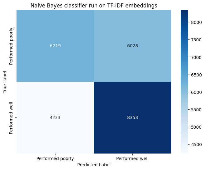
Fig.42 Naive Bayes Confusion Matrix
The results suggest that while the model wasn't able to capture all the patterns between the 'titles' feature and the 'views/elapsedtime' feature from the dataset, it did demonstrate the existence of some patterns. With accuracy, precision, and recall hovering around 58%, the model performed better than random guessing. However, it falls short of being able to make meaningful predictions due to inadequate training on the dataset.
These outcomes align with expectations for Naive Bayes classifiers, which are basic probabilistic classifiers lacking the advanced capability to discern complex patterns present in text documents. While unsupervised learning algorithms and Naive Bayes have indicated a relationship between YouTube titles and their corresponding views, more sophisticated algorithms such as CNN or LSTM could better capture and learn intricate patterns from the dataset. These advanced models are adept at handling sequential data like text and could potentially yield more accurate predictions by extracting deeper insights from the 'titles' feature in relation to 'views/elapsedtime'.
Decision trees (refer Figure 43) are supervised machine learning algorithms, suitable for both classification and regression tasks. The algorithm operates by partitioning the dataset's features into smaller sets with the help of input features, aiming to predict the output feature. The model trains itself by adjusting the decision of splits at each node, aiming to find the best split using either the Gini Index or Information Gain.
Entropy measures the amount of disorder or uncertainty in the dataset, the formula is provided in Figure 45. It is commonly used in making decisions at nodes in the decision trees. Entropy minimization is the aim while making decisions on a decision tree. Maximum entropy would mean that the classes are evenly distributed and consist of maximum disorder.
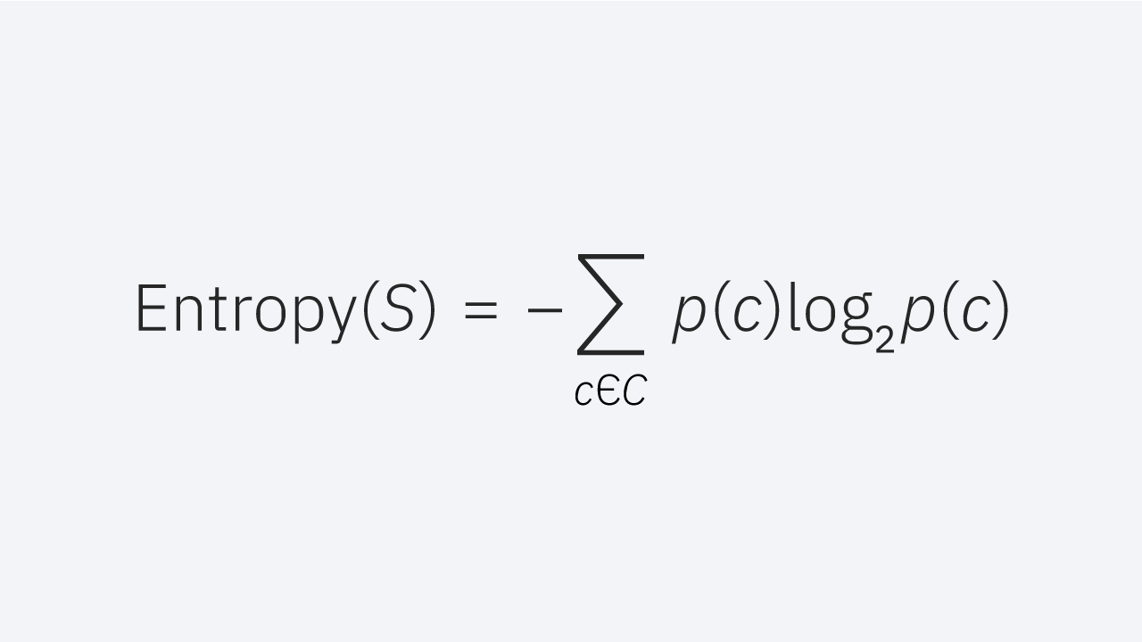
Entropy formula (Fig. 45)

Information Gain formula (Fig. 46)
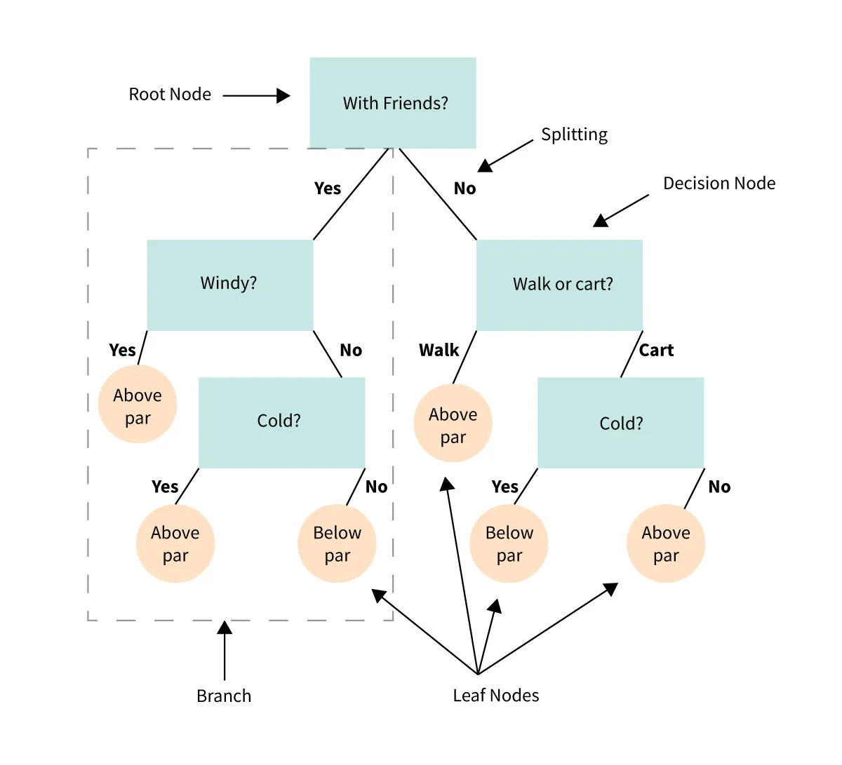
Decision Tree Example (Fig. 43)

Gini Index formula (Fig. 44)
Information Gain quantifies the amount of information or pattern a particular subset of data would capture if it's split at that particular node, which measures the reduction in entropy achieved by a split. Entropy (refer Figure 45) measures the amount of disorder or uncertainty in the dataset. The main aim of the method is to reduce the uncertainty such that the model is able to learn patterns in the dataset. Higher the information gain the better is the split. The formula for the same is given in Fig. 46. While this particular project aims at utilizing Gini Index as the split parameter, many applications use Information Gain and entropy to make decisions.
The process of making predictions for testing is fairly simple: the tree is traversed from the root node by making decisions at each internal node based on the feature values of the data point and the splitting parameter (Gini Index in our case). The prediction is the value obtained at the final node, which is the leaf node.
The data preparation stage of decision tree classifier was conducted in multiple steps,
Click on each of the images below to view the sample dataset in each category.

Fig.25 Sample of Original Cleaned Data
The Decision Tree Model was trained on the training dataset, and the results were obtained from the testing dataset and visualized in Figure 49. Analysis of the visualization reveals that both the accuracy and recall metrics, derived from both BERT and SpaCy embeddings, achieved scores in the vicinity of 55%. Initially trained with the default 'max_depth' parameter, the model exhibited signs of overfitting, evident from the complex tree structure observed in Figure 50. However, upon adjusting the 'max_depth' parameter to 5, the model demonstrated improved fitting to the dataset, as depicted in Figure 51 (a) and Figure 51 (b).
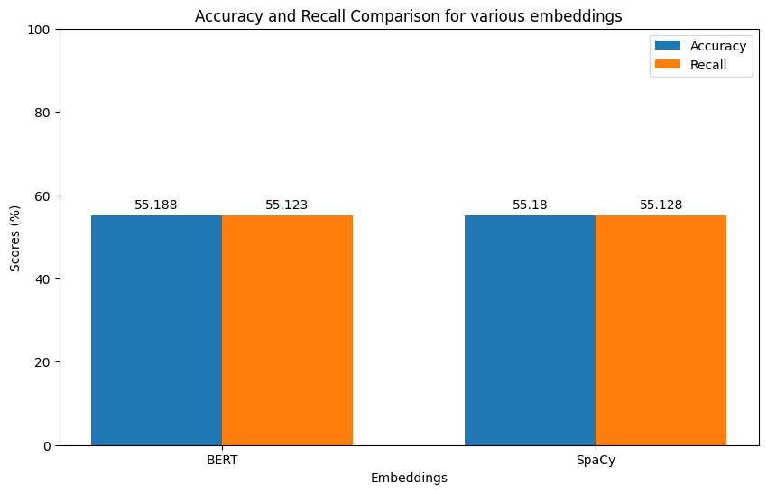
Decision Tree evaluation metric (Fig. 49)
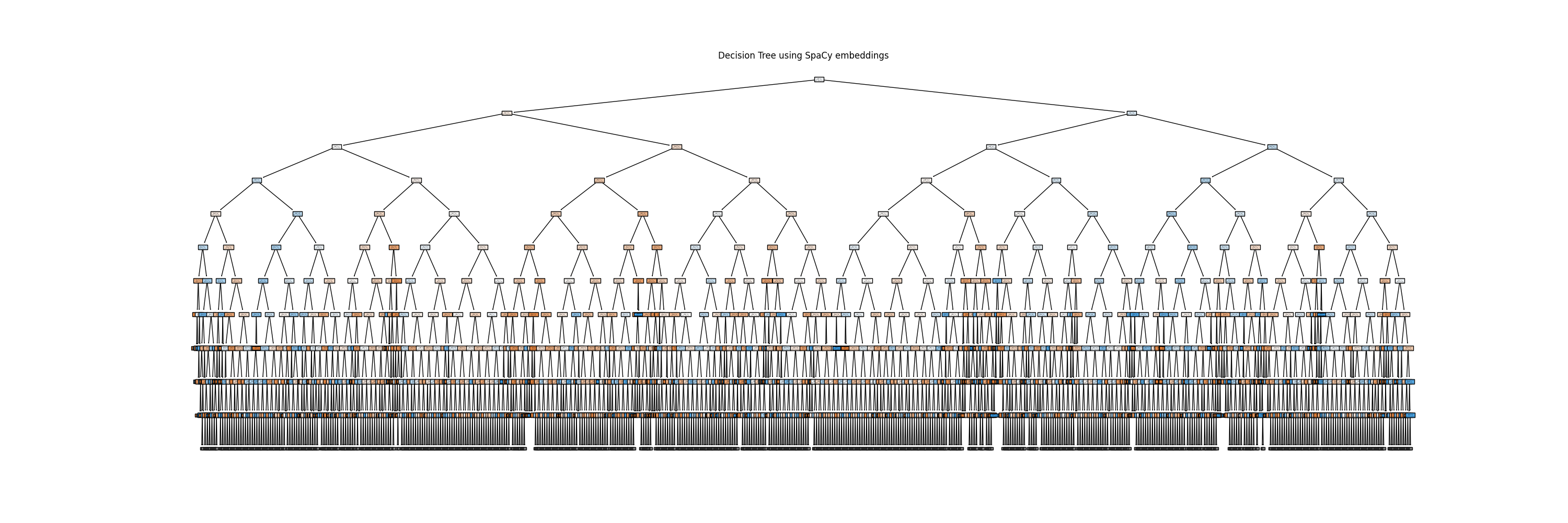
Initial Decision tree (Fig. 50)
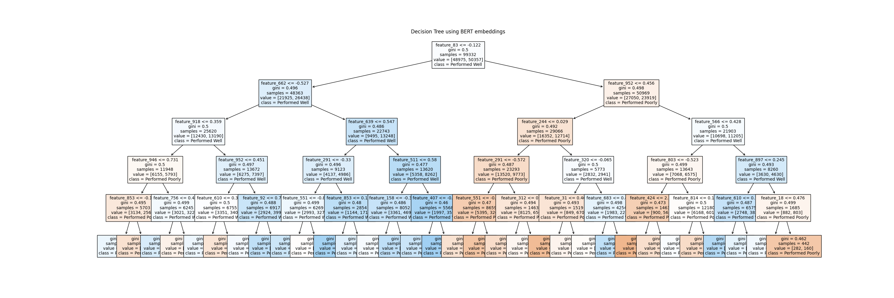
Decision Tree using BERT Embeddings (Fig. 51 (a))

Decision Tree using SpaCy Embeddings (Fig. 51 (b))
Furthermore, examination of the confusion matrix, Fig. 52 (a) and Fig. 52 (b) from both embeddings indicates an even distribution of both labels throughout the matrix. This uniform distribution suggests that the model effectively learned both features with equal proficiency.
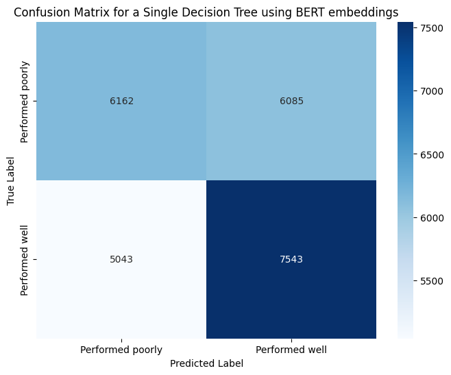
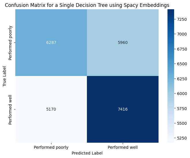
Confusion Matrix for BERT and SpaCy Embeddings DT (Fig. 52 (a) and Fig. 52 (b))
In conclusion, the experiment revealed that the decision tree classifier struggled to effectively train on the dataset due to its complexity. Nonetheless, the findings suggest the presence of a discernible pattern between YouTube video titles and their corresponding views over time. Although setting the 'max_depth' parameter to 5 helped prevent overfitting, it did not significantly improve model accuracy on the test dataset.
The experiment, conducted using both BERT and SpaCy embeddings, aimed to observe any differences in predictions. Surprisingly, both embeddings performed similarly, indicating that the decision tree classifier may not effectively leverage the advanced linguistic characteristics captured by BERT. This suggests that the decision tree classifier may not be the optimal model for capturing the complex patterns within text documents. Moving forward, it is evident that employing more advanced models like CNN or LSTMs may yield better classification results by effectively leveraging the intricate linguistic features present in the text.
Support Vector Machine (SVM) (refer Fig. 53) is one of the most advanced supervised machine learning algorithms, known for its capability in creating decision boundaries around complex classes. SVMs excel when the classes are separable, and a clear boundary can be defined between them. The primary goal of SVM is to find the hyperplane that maximizes the margin between these classes.
Kernels, as mentioned earlier, are used in situations where the classes are not linearly separable (Refer to Fig. 55). Kernels help in transforming the input data to a higher dimension in the hope of finding a linear separator in that space. Kernels are fascinating functions because they allow SVMs to compute the decision boundary in the original feature space as if it were a higher-dimensional space. Kernels are specific types of functions that compute the dot product efficiently without explicitly transforming the data into the higher-dimensional space.
The dot product is extremely helpful in kernels because it leverages the fact that SVMs only need to calculate the dot product between data points in the feature space, avoiding the explicit computation of vectors in a higher-dimensional space. Kernels compute the dot product directly in the higher-dimensional space, thereby reducing the complexity of calculations and allowing for efficient computation without the need for explicit transformation.
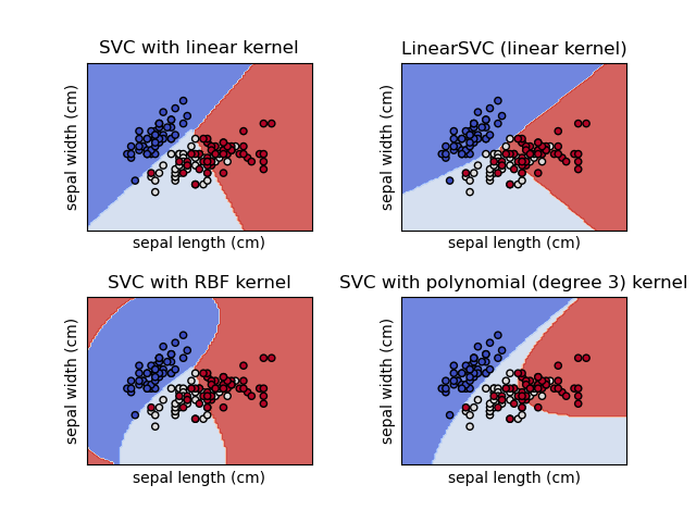
SVM classifier on various kernels (Fig. 55)
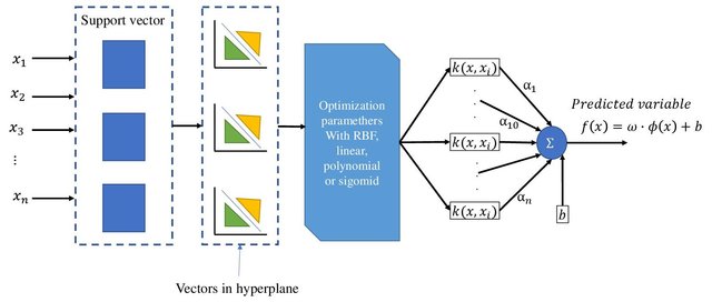
SVM Architecture (Fig. 53)
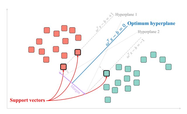
An SVM example for linearly separable (Fig. 54)
The Polynomial Kernel function (Refer Fig. 56) computes a dot product between the input vectors in the original feature space and raises the sum by the specified degree d. The constant c allows for shifting the polynomial. On the other hand, the Radial Basis Function (RBF) Kernel (Refer Fig. 56) measures the similarity between vectors based on the Euclidean distance. An example is presented in Fig. 56 to illustrate the casting of 2D points into 6D points using a polynomial kernel.
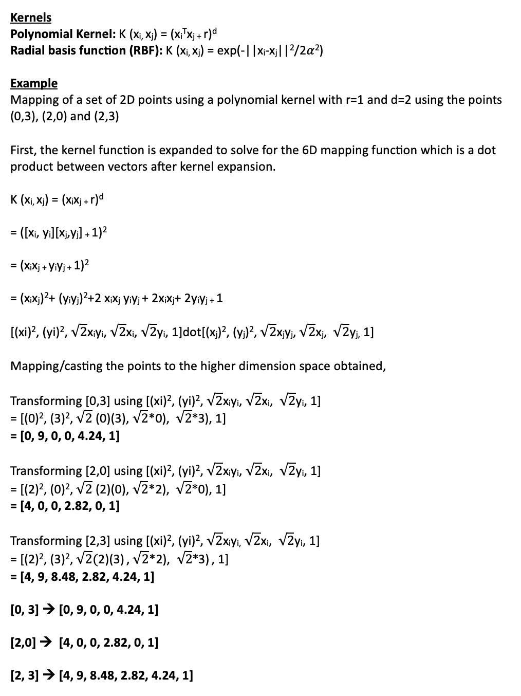
Kernels and Example (Fig. 56)
The data preparation stage began with, collecting thumbnail URLs using a YouTube API request (refer to Fig. 57), followed by extracting the thumbnails using another Google Drive API request (refer to Fig. 58). Subsequently, the thumbnails were pre-processed using the VGG16 neural network to extract the most important features from the images. The output of the VGG16 network was then stored in a numpy file to be used as input for the SVM model. The model is then trained to predict if the thumbnails would fall into the category of the video performing well or performing poorly. The link to the dataset can be found here. The link to the sample thumbnails extracted can be found here.
Click on each of the images below to view the sample dataset in each category.

Fig.57 Sample of Original Cleaned Data

Fig.58 Sample of thumbnails extracted
The code to Support Vector Machine Classifier performed on python can be found here: SVM.
The output of VGG16 was used as input for various SVM models fine-tuned with different kernels and C values. These models were evaluated based on precision, accuracy, recall, and F1-score. The results obtained were compiled into a table, as shown in Table 1. Confusion matrices for the SVM models can be found in Figures 59, 60, 61.
It was observed that the RBF kernel with a C value of 1 yielded the best result, achieving an accuracy of 60%, precision of 62%, recall of 60%, and F1-score of 61%. These results are depicted in Figure 62. The linear kernel performed next best, consistently achieving similar results across different C values, with an accuracy of 56%, precision of 58%, recall of 57%, and F1-score of 57.5%. The polynomial kernel performed the least favorably, with the highest scores achieved at a C value of 10, resulting in an accuracy of 59%, precision of 63%, recall of 48%, and F1-score of 54%. Despite exhibiting higher precision and accuracy, the polynomial kernel tended to underfit the data.
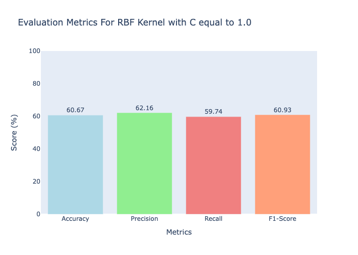
SVM evaluation metric (Fig. 62)
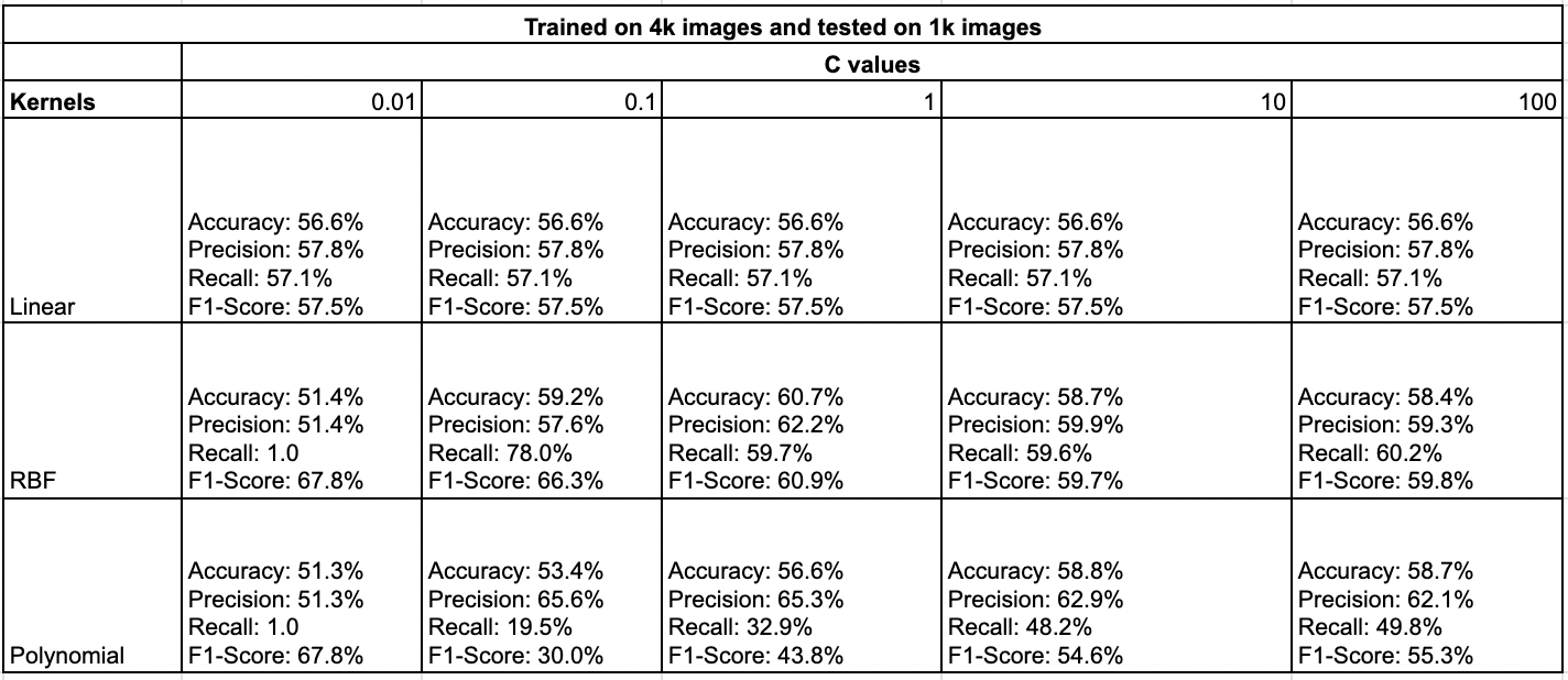
SVM classifier on various kernels (Table. 1)
In conclusion, the evaluation of SVM models with various kernels and C values using VGG16-extracted features has provided insights into their performance on image classification tasks. Among the experiments conducted, the RBF kernel with a C value of 1 emerged as the winner, exhibiting strong overall performance with balanced accuracy, precision, recall, and F1-score metrics. The consistent performance of the linear kernel across different C values highlights its reliability for this task. However, the polynomial kernel, particularly at higher C values, showed signs of potential overfitting or underfitting, this shows the importance of careful parameter selection.
To explore the captivating world of YouTube titles and thumbnails and their impact on views, this study delves deep into how these aspects can influence video performance over time. By analyzing these factors, valuable insights are uncovered on how to improve channel performance. Firstly, the research reveals patterns regarding the impact of title length on video performance, noting that longer titles tend to attract higher viewership (refer Fig. 61) compared to shorter ones (refer Fig. 62). This suggests that while attention-grabbing titles are crucial, providing a sufficiently detailed title is also essential to attract viewers. Additionally, there is a direct correlation between title length and video performance metrics such as likes, comments, and subscribers gained.
Moreover, the study highlights the significance of visual appeal through thumbnail design, showing that careful thumbnail design is vital for enhancing video performance. Specific colors, images, or styles may be more effective in capturing viewer interest and encouraging clicks on the video (refer Fig. 63,64). The interplay between titles and thumbnails plays a crucial role in attracting views, with effective thumbnails that complement the title contributing to higher view counts. Certain combinations of thumbnails and titles may perform exceptionally well by increasing viewership and setting clear expectations about the video content. Therefore, crafting a compelling title and thumbnail is considered the initial step towards a successful video.

Fig. 63 Attractive Thumbnail

Fig. 64 Attractive Thumbnail Example 2

Fig. 61 Short Title

Fig. 62 Long Title
The relationship between the recommendation system and optimizing titles and thumbnails is another intriguing aspect. As titles and thumbnails directly impact the number of views a video gains, they likely influence the recommendation system, which heavily relies on video click-through rates. Understanding peak viewer activity times can help optimize content release schedules for maximum visibility and engagement. Additionally, demographic factors play a role in viewer preferences for thumbnails and titles. Different audience segments may respond differently to specific colors, images, or content styles, highlighting the importance of audience segmentation and targeting in content creation.
Future studies could focus on developing advanced systems to learn the combinations of titles and thumbnails that attract views. By employing such advanced systems, YouTube content creators can benefit from crafting appropriate titles and thumbnails for their videos. Analyzing the impact of click-through rates on video performance, rather than absolute view counts, can provide insights into video recommendation system behavior. Furthermore, assessing the relationship between views and video duration can improve video content and overall performance. The field of youtube has so much potential for analysis with all the numbers that flow in every second from videos around the world. Conducting future research in the field and carefully examining the nature of the titles and thumbnails can bring our analysis not just in the field of youtube but also a general understanding of the human brain by learning the patterns that tend a youtube recommendation to be converted to a view.
In conclusion, the findings underscore the importance of both the art and science behind video content creation on YouTube.Effective thumbnail design, aptly summarized by the saying 'A picture is worth a thousand words', along with compelling titles and a profound understanding of viewer behavior, serves as the cornerstone for enhancing video performance and fostering audience engagement. This holistic approach to content optimization opens up new opportunities for creators to connect with their audiences and thrive in the dynamic world of digital content. Furthermore, the insights gained from this analysis are not limited to content creators alone; they also hold significant potential for advertisements and marketing strategies. By identifying patterns in visual elements that attract attention, advertisers and marketing professionals can leverage this knowledge to attract more customers to their products or services. UX designers can also apply the findings from this research study of effective content creation by improving the user experience. By considering factors such as titles and thumbnails designs, the designers can get much more creative in creating engaging user interfaces attracting human attention.
Rohit.Raju@colorado.edu
1600 Amphitheatre Parkway
Mountain View, CA
94043 US